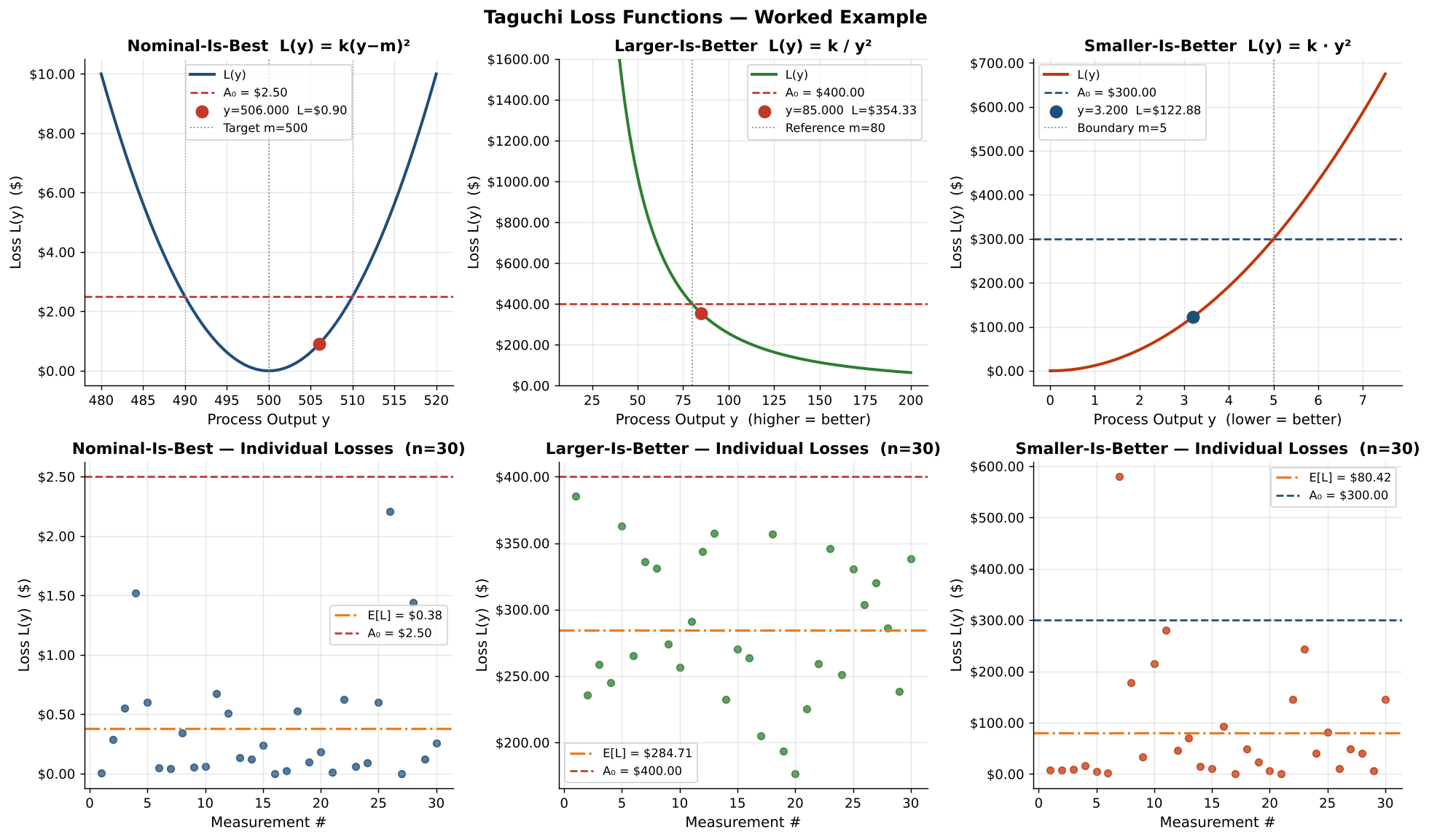
Put a dollar figure on variation — not just on scrap. Calculate quality loss for a single part or a whole batch, then download the same calculator as an Excel workbook, Python or R, with a worked example.
A part at the spec limit and a part just inside it are nearly the same part. Taguchi's quadratic loss reflects that: cost grows smoothly as output drifts from ideal, instead of jumping from $0 to scrap at the limit.
NIB
Nominal-Is-Best
L(y) = k(y − m)² k = A₀ / Δ²
A target value is ideal and deviation either way costs money. Diameters, fill weights, voltages.
LIB
Larger-Is-Better
L(y) = k / y² k = A₀ · m²
More is always better. Bond strength, tensile strength, efficiency, life to failure.
SIB
Smaller-Is-Better
L(y) = k · y² k = A₀ / m²
Zero is ideal. Leak rate, wear, shrinkage, noise, contamination, wait time.
A₀ = cost to the customer or business when output reaches the tolerance / reference point (rework, warranty, give-away). Δ = tolerance half-width. m = target (NIB) or reference limit (LIB/SIB).
// Interactive
Loss calculator
Pre-loaded with the worked example. Change the inputs or paste your own measurements — one per line, or comma-separated straight from Excel.
k constant
–
L(y) single
–
E[L] per unit
–
Batch total
–
–
From spread From off-target
Loss curveA₀ limitBatch pointsSingle y
// Download. Open. Analyze.
Run it on your own data
The Excel, Python and R versions give identical results to the cent. Both read CSV or Excel, print a summary, plot the curve and individual losses, and export per-part results.
Preview before you downloadEvery file opens in a viewer first, so you can read the code or see what's inside before anything touches your computer.
Plain text and formulas onlyThe .py and .R files are readable source code. The workbook is .xlsx, a format that cannot contain macros.
Check the fingerprintEach preview shows the file's SHA-256 checksum, also listed in SHA256SUMS.txt and matched by the public source on GitHub.
terminal / python
# install once
pip install numpy pandas matplotlib

# run the worked example (prints summaries, saves taguchi_example_python.png)
python taguchi_loss.py demo

# single part
python taguchi_loss.py nib --target 500 --delta 10 --A0 2.50 --y 506

# batch from your CSV, save the chart and per-part results
python taguchi_loss.py nib --target 500 --delta 10 --A0 2.50 \
    --csv example_data.csv --column fill_weight_g --save nib.png --export nib_results.csv

# or use it as a library
from taguchi_loss import NominalIsBest
nib = NominalIsBest(target=500, delta=10, A0=2.50)
print(nib.from_csv("example_data.csv", "fill_weight_g").summary())
R / RStudio
# from a terminal: run the worked example (saves taguchi_example_R.png)
Rscript taguchi_loss.R demo

# inside R or RStudio
source("taguchi_loss.R")
nib <- taguchi_calc("nib", target = 500, delta = 10, A0 = 2.50)
taguchi_eval(nib, 506)                                   # single part

b <- taguchi_from_csv(nib, "example_data.csv", "fill_weight_g")
print(b)                                                 # batch summary
taguchi_plot(nib, b)                                     # curve + losses
taguchi_export_csv(b, "nib_results.csv")

lib <- taguchi_calc("lib", m = 80, A0 = 400)
sib <- taguchi_calc("sib", m = 5,  A0 = 300)
// Worked example
One line, three characteristics
A packaging line measures 30 units for fill weight, seal bond strength and leak rate. These are the results the workbook and both scripts produce from example_data.csv.
Characteristic
Type
Spec / A₀
Mean
E[L] / unit
Batch (30)
Status
Fill weight (g)
NIB
500 ± 10 · $2.50
502.49
$0.38
$11.46
Acceptable — 41% of loss is off-target
Bond strength (MPa)
LIB
≥ 80 · $400
96.20
$284.71
$8,541.19
Caution — E[L] > 50% of A₀
Leak rate (ccm)
SIB
≤ 5 · $300
2.06
$80.42
$2,412.74
Acceptable — 1 unit over limit
Reading it: fill weight is fine, but re-centring the filler from 502.5 g to 500 g removes about 41% of its loss for free. Bond strength passes spec on every unit yet carries the largest cost — a capability problem that a pass/fail view hides.